Worked example · Statistics

Normal distribution probability: mean 70, standard deviation 8

Scores on a test are modelled by a normal distribution with mean 70 and standard deviation 8. What proportion lie from 62 to 78, and what proportion exceed 86? The arithmetic starts with a z-score, but the answer is an area. That distinction is the difference between reading a bell curve and merely finding its height.

A-level
Ans calculator
Ans Graph
Numerical integration
≈ 8 minutes

Step 1 — on paper

Turn the raw scores into z-scores

A z-score measures distance from the mean in standard deviations. For a value x from a distribution with mean μ and standard deviation σ:

z = \frac{x - μ}{σ}

x raw score · μ mean, 70 · σ standard deviation, 8 · z signed distance from the mean in standard deviations

The lower limit 62 is one standard deviation below 70, and the upper limit 78 is one above:

z_{62} = \frac{62 - 70}{8} = - 1 z_{78} = \frac{78 - 70}{8} = 1

So the question is the familiar central band from z = −1 to z = 1. A rough empirical-rule answer is about 68%. The full normal model gives 0.6826894921, or 68.27%.

Step 2 — set the scale

The bell curve's height is not the probability

The probability density for this model is f(x) = e^{−(x−70)²/(2×8²)} ÷ (8√(2π)). At the mean the exponential part is e⁰ = 1, so the maximum height is just:

1
÷
(
8
×
√
2
×
π
)
)
=

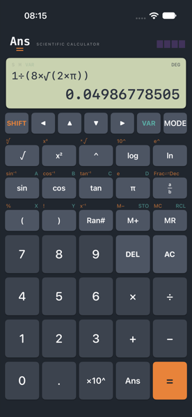
1÷(8×√(2×π)) 0.04986778505 The curve's peak density at x = 70 — not a 4.99% probability

Ans on iPhone showing 1 divided by, open bracket, 8 times the square root of 2 times pi, close bracket, and the result 0.04986778505. — The density has units of probability per score unit. Only an area over an interval is a probability.

A single exact score has probability zero in a continuous model. The curve height tells us how densely probability is packed nearby. It takes width as well as height — the area under the curve — to produce a non-zero probability.

Step 3 — on the graph

Shade the probability from 62 to 78

Enter the density and set a window that shows the whole bell — x from 40 to 100 and y from 0 to 0.055 is the one below. Then choose Integral with lower bound 62 and upper bound 78:

f₁(x) = e^(-0.5*((x-70)/8)^2)/(8*sqrt(2*pi))

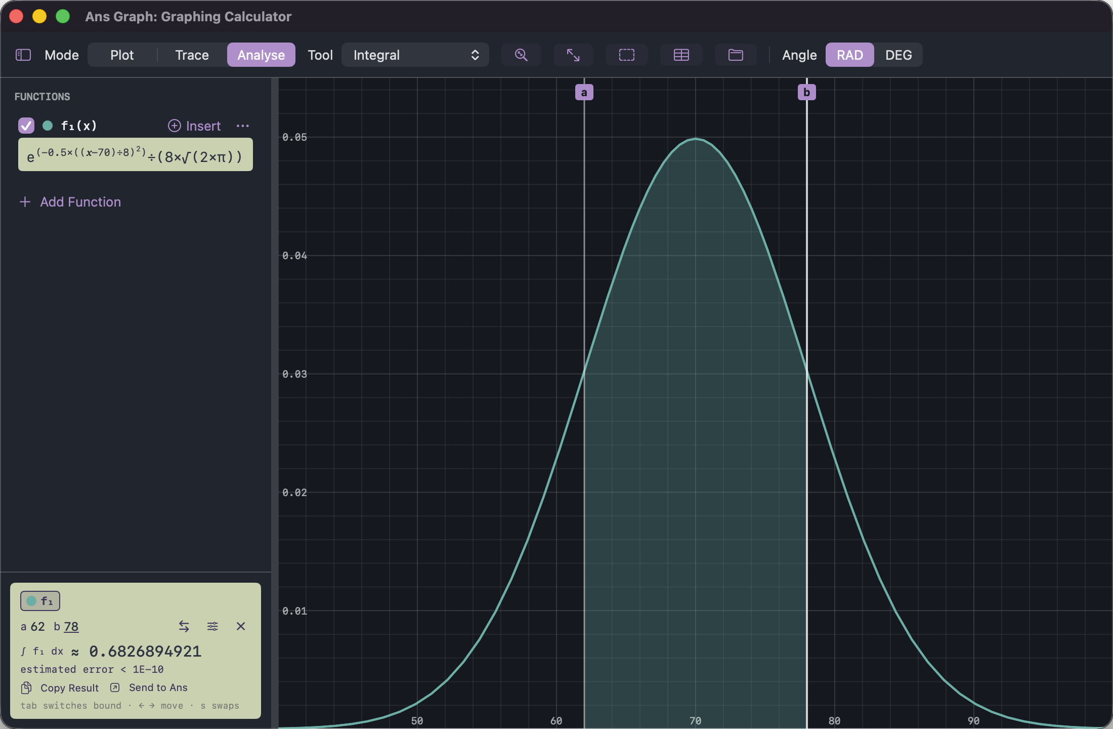
Ans Graph showing a normal bell curve centred at 70, with the area from 62 to 78 shaded and the integral read as 0.6826894921. — **Integral 62 to 78** — the register reads **0.6826894921** with an estimated error below 10⁻¹⁰: the same ten digits as the exact value in Step 1, so about 68.27% of the modelled scores lie within one standard deviation of the mean.

Symmetry provides a second check. Exactly half the distribution lies on either side of 70, and the intervals 62–70 and 70–78 must have equal area. Each side therefore contributes 0.3413447461.

Step 4 — a tail probability

What proportion scores above 86?

Standardise 86 first: (86−70)÷8 = 2, so the cutoff is two standard deviations above the mean. The central area from z = −2 to z = 2 is 0.9544997361. The remaining probability is split equally between the two tails:

P (X > 86) = \frac{1 - 0.9544997361}{2} = 0.02275013195

The model predicts 2.275% above 86. In 1,000 independent scores that is an expected count of about 23, not a promise that every group of 1,000 will contain exactly 23.

Central coverage of a normal distribution.
Raw interval	z interval	Modelled probability
62 to 78	−1 to 1	0.6826894921 (68.27%)
54 to 86	−2 to 2	0.9544997361 (95.45%)
46 to 94	−3 to 3	0.9973002039 (99.73%)
above 86	above 2	0.02275013195 (2.275%)

What the normal model assumes

The score distribution is adequately described by a symmetric normal curve. Real tests can be skewed, capped or multi-modal.
The mean 70 and standard deviation 8 are treated as known population parameters rather than estimates with uncertainty.
Scores are treated as continuous. If only integer scores are possible, a continuity correction may be required for a discrete probability.
The model can assign probability below or above physically possible score limits; that matters when the mean is near a boundary.
Expected proportions describe repeated samples, not a guaranteed count in one class or one sitting.

Next: the gradient of a curve for another distinction between a point value and an interval, or area under a velocity–time graph for integration with physical units.

Free
No ads
No tracking
No account
Every sum shown in full

Worked on Ans — a scientific calculator you can own for the z-scores and density, and Ans Graph for the probability area. Both are paid for once and work offline.