Worked example · Physics

Area under a velocity–time graph, when it isn't a triangle

The area under a speed–time graph is the distance travelled. At GCSE that area is made of rectangles and triangles and you can find it with a ruler. This page does that case properly, then breaks it twice: once with a car whose drag grows with speed, and once with a rocket that is burning away its own mass. Both are still speed–time graphs. Neither has a triangle in it.

GCSE to A-level
Ans calculator
Ans Graph
≈ 9 minutes

Step 1 — on paper

The easy case: how to find distance from a velocity–time graph

A vehicle travels at a steady 8 m/s for 3 seconds, then brakes evenly and stops 2 seconds later. How far has it gone?

Speed–time or velocity–time? Everything on this page travels one way, so the two graphs are the same picture and the area under them is the distance travelled. They part company the moment something reverses: on a velocity–time graph the part below the axis counts as negative, and the area then gives displacement — where the object ended up — rather than how far it went. Ans Graph's integral signs its answer the same way, which is what the swap control on the register is for.

Split the area into shapes you know. Under the flat part is a rectangle; under the braking part is a triangle:

Rectangle 8 × 3 = 24 m, triangle ½ × 2 × 8 = 8 m. Total 32 m.

On the calculator that is one line — and worth typing as one line, because breaking it up is how the halving gets applied to the wrong term:

(
8
×
3
)
+
(
0.5
×
2
×
8
)
=

(8×3)+(0.5×2×8) 32 The distance travelled, in metres

No app is needed for this step, and none is offered. A shape made of straight lines is a ruler-and-arithmetic problem. Ans Graph plots y = f(x) — one continuous expression — so a graph made of two separate straight pieces is not what it is for. It becomes the right tool exactly when the line stops being straight, which is the next step.

Step 2 — where the triangle lies

A real car does not accelerate in a straight line

Put your foot down in a real car and the acceleration falls away as you speed up. Air resistance grows with speed, so the net force shrinks, and the speed–time graph bends over towards a top speed instead of climbing forever. Taking the drag as proportional to speed gives the standard first-order model:

v (t) = v_{\infty} (1 - e^{- t / τ})

v∞ the top speed it approaches but never reaches · τ the time constant: how quickly it gets there · t time from a standing start

Take v∞ = 45 m/s (just over 100 mph) and τ = 8 s. That car passes 60 mph in 7.25 seconds, which is ordinary for a family car, and at ten seconds it is doing 32.11 m/s — about 72 mph.

So: how far has it gone in those ten seconds? The GCSE instinct is a triangle from 0 to 32.11 m/s, giving ½ × 10 × 32.11 = 160.54 m.

That is wrong, and not by a little. The real curve sits above the straight line for the whole ten seconds — the car does most of its accelerating early — so a triangle under-counts every metre of that gap. The true answer is 193.14 m. The triangle is out by 32.6 metres, about seven car lengths, on a ten-second measurement.

Step 3 — the area under a curve

Integrating the speed–time curve

Distance is the area under the curve whatever shape the curve is; the only question is how you find the area. Three ways, and they should agree.

By hand: the trapezium rule

Slice the ten seconds into five strips of 2 s, take the speed at each boundary, and treat each strip as a trapezium. Read the speeds off the formula: 0, 9.954, 17.706, 23.744, 28.445 and 32.107 m/s. Then distance ≈ 2 × [½(0 + 32.107) + 9.954 + 17.706 + 23.744 + 28.445]:

2×(0.5×(0+32.107284)+9.954+17.7061+23.7435+28.4454) 191.805284 Close, and slightly under — the curve bulges above every chord

On the graph: the area, shaded

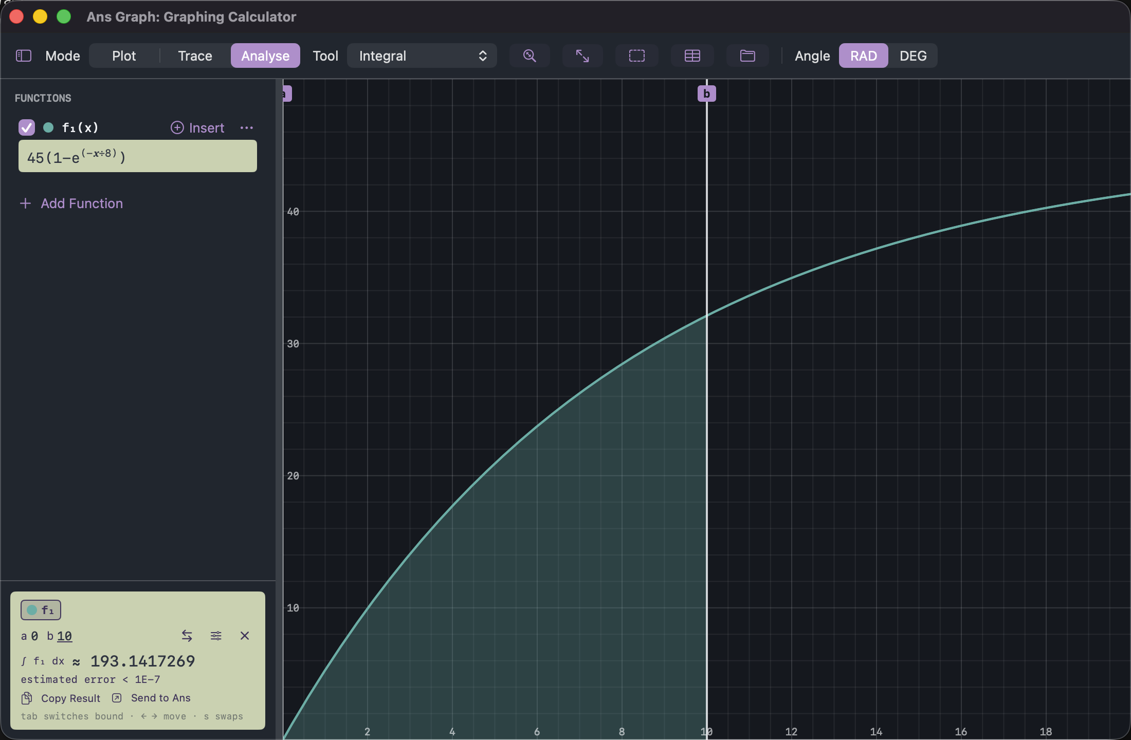
Type the model straight in, with time as x:

f₁(x) = 45(1−e^(−x/8))

Choose Integral, set the bounds to 0 and 10, and the region under the curve is shaded with its value beside it — 193.1417269, agreeing with the closed form below to every digit it prints. Drag either bound and both the shading and the number follow, so "how far between the fourth and seventh second?" is a gesture rather than a new calculation.

Ans Graph: a speed curve rising steeply then flattening towards 45 metres per second, with the area from 0 to 10 seconds shaded and the register reading approximately 193.14 with an estimated error beneath it. — The shaded area is the distance travelled: **193.1417269 m**, with **estimated error < 1E−7** printed beneath it rather than hidden.

Exactly: the closed form

This particular integral can be done by hand, which makes it a good test of the other two. Integrating the model term by term:

s = \int_{0}^{T} v (t) d t = v_{\infty} [T + τ (e^{- T / τ} - 1)]

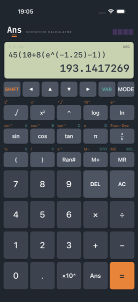
With T = 10, v∞ = 45 and τ = 8 — note e^x is the SHIFT function of the ln key:

45
(
10
+
8
(
SHIFT
e^
−1.25
)
−
1
)
)
=

45(10+8(e^−1.25−1)) 193.1417269 The exact answer, to ten significant figures

Ans on iPhone showing 45(10+8(e^(−1.25)−1)) on the input line and 193.1417269 as the result. — The closed form on the phone — the number against which the shaded area and the trapezium rule are both judged.

Three methods, one distance. Only one of them claims to be exact.
Method	Distance	Error
Triangle (uniform acceleration)	160.54 m	−32.61 m
Trapezium rule, 2 s strips	191.81 m	−1.34 m
Ans Graph integral	193.1417269 m	stated as < 1E−7
Closed form	193.1417269 m	exact

The trapezium rule is out by 1.34 m because every straight chord cuts the corner off a curve that bends downwards. Halve the strips to 1 s and it improves to 192.81 m — still under, and still converging from the same side. That systematic direction is worth more than the number: an error you can predict the sign of is one you can allow for.

Step 4 — constant thrust in space

When even the acceleration will not sit still

A spacecraft coasting far from anything fires its engine at constant thrust. Nothing is slowing it down, so surely the speed–time graph is the straight line from GCSE — constant force, constant acceleration?

No, because it is throwing its own mass out of the back. As the propellant burns the vehicle gets lighter, so the same thrust produces more acceleration every second, and the graph curves upwards. The speed at time t is Tsiolkovsky's rocket equation:

v (t) = v_{e} \ln (\frac{m_{0}}{m_{0} - \dot{m} t})

vₑ exhaust speed · m₀ starting mass · ṁ mass burned per second · t time since ignition

Take a 2,000 kg craft, an exhaust speed of 3,000 m/s, and 2 kg of propellant a second for 500 seconds — half its mass gone in a little over eight minutes. Plot the truth against the straight line that a fixed-mass assumption predicts, where a = vₑṁ/m₀ = 3 m/s²:

f₁(x) = 3000×ln(2000/(2000−2x)) f₂(x) = 3x

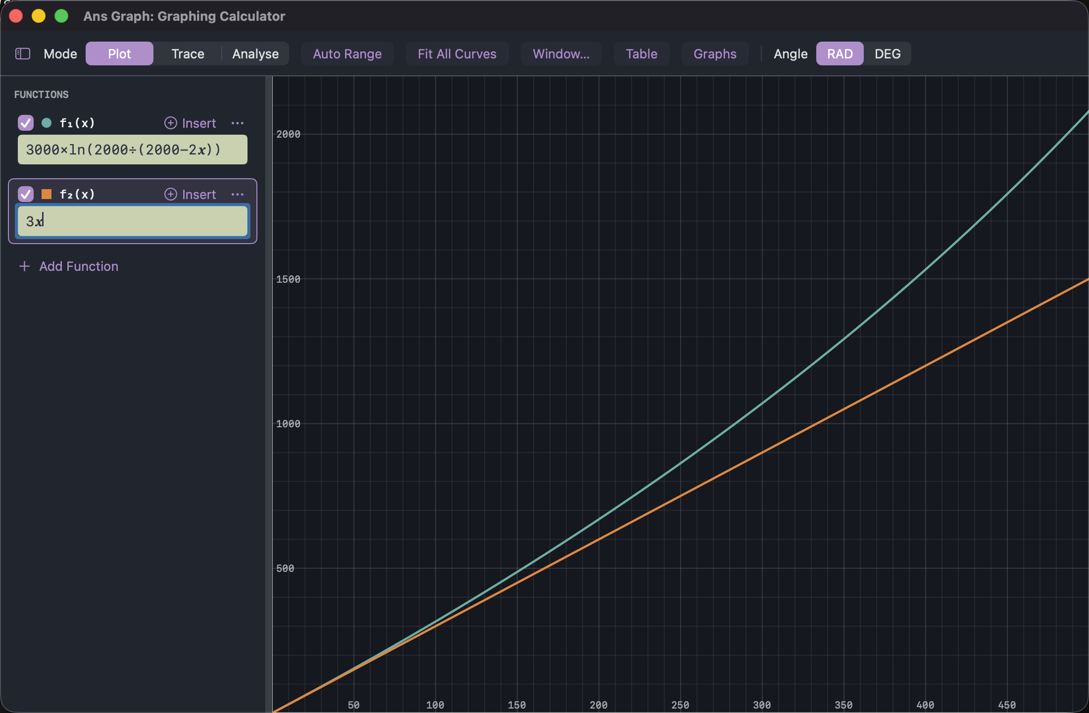
Ans Graph: a curve bending upwards to about 2,079 metres per second at 500 seconds, plotted against a straight line reaching only 1,500 metres per second. — Constant thrust, falling mass: **2,079 m/s** after the burn, against the **1,500 m/s** the straight line predicts.

And the distance covered is, as ever, the area underneath. Shading it from 0 to 500 gives 460.3 km, where the straight line's triangle gives ½ × 3 × 500² = 375 km. Assuming constant acceleration would put the craft 85 kilometres short of where it actually is, after one eight-minute burn.

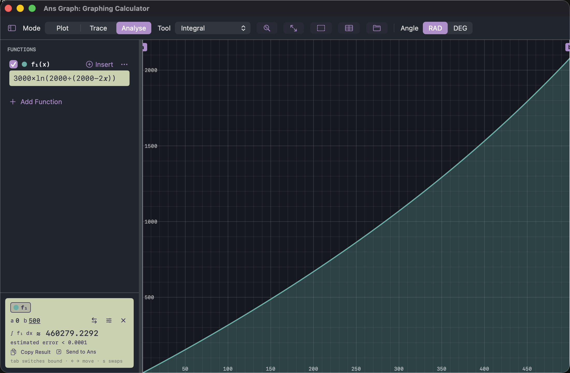
Ans Graph: the area under the rocket's speed curve from 0 to 500 seconds shaded, with the register reading approximately 460,279 metres. — The area under the curve: **460,279 m** travelled during the burn.

Watch the far end of that curve. Push the upper bound towards 1,000 seconds and the model claims infinite speed — at t = 1,000 the craft has burned all 2,000 kg of itself and the logarithm's argument goes to zero. A model is only ever quoted inside the range where its assumptions hold, and the graph makes the edge of that range visible instead of leaving it in a footnote.

Check your own numbers

The car, second by second

v = 45(1 − e^−t/8). Set the Ans Graph table to start 0, step 2 and compare the column.
t / s	v / m s⁻¹	v / mph	Distance so far / m
0	0.000	0.0	0.00
2	9.954	22.3	10.37
4	17.706	39.6	38.35
6	23.744	53.1	80.05
8	28.445	63.6	132.44
10	32.107	71.8	193.14

What these models ignore

Step 1 assumes the braking is perfectly even, so the sloping section really is a straight line. Real brakes are not, though they are close enough for the mark scheme.
The car model takes drag as proportional to speed. Above walking pace real air resistance goes more like the square of speed, so the curve is a teaching model rather than a road test; the shape and the argument are right, the exact metres are not a measurement.
Gear changes, wheelspin, gradient, wind and the driver are all absent from a two-parameter model.
The rocket is in free space with no gravity and no drag, at constant thrust and constant mass flow. Launch from a planet adds gravity losses, which is why real launch profiles are not this curve.
Numerical integration is an estimate with a stated uncertainty. Where an exact closed form exists — as it does for both curves here — it is the thing to check against.

Next: compound interest, where the same exponential runs the other way, or mortgage repayments.

Free
No ads
No tracking
No account
Every sum shown in full

Worked on Ans — a scientific calculator you can own and Ans Graph, whose shaded integral with draggable bounds is the interaction step 3 is built around.